16. Mean filters
This example compares the following mean filters of the rank filter package:
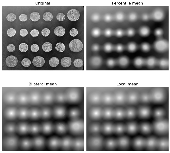
16.1. local mean:
all pixels belonging to the structuring element to compute average gray level.
16.2. percentile mean:
only use values between percentiles p0 and p1 (here 20% and 80%).
16.3. bilateral mean:
only use pixels of the structuring element having a gray level situated inside g-s0 and g+s1 (here g-200 and g+200)
Percentile and usual mean give here similar results, these filters smooth the complete image (background and details). Bilateral mean exhibits a high filtering rate for continuous area (i.e. background) while higher image frequencies remain untouched.
import matplotlib.pyplot as plt

from skimage import data
from skimage.morphology import disk
from skimage.filters import rank
16.4. Load
image = data.coins()
selem = disk(20)
16.5. Mean filters
percentile_result = rank.mean_percentile(image, selem=selem, p0=.2, p1=.8)
bilateral_result = rank.mean_bilateral(image, selem=selem, s0=200, s1=200)
normal_result = rank.mean(image, selem=selem)
16.6. Show
fig, axes = plt.subplots(nrows=2, ncols=2, figsize=(10, 10),
                         sharex=True, sharey=True)
ax = axes.ravel()

titles = ['Original', 'Percentile mean', 'Bilateral mean', 'Local mean']
imgs = [image, percentile_result, bilateral_result, normal_result]
for n in range(0, len(imgs)):
    ax[n].imshow(imgs[n], cmap=plt.cm.gray)
    ax[n].set_title(titles[n],fontsize=16)
    ax[n].axis('off')

plt.tight_layout()
plt.show()